safehaven: Hedge and Safe Haven Testing in R

A getting-started guide to hedge and safe-haven analysis with the safehaven R package.

The safehaven package tests the hedge and safe haven hypotheses (Baur, D. G., T. K. McDermott, 2010), estimates hedge ratios, hedging effectiveness and optimal portfolio weights (Basher, S. A., P. Sadorsky, 2016), and computes the conditional diversification benefit (Christoffersen, P., V. Errunza, K. Jacobs, H. Langlois, 2012; Christoffersen, P., K. Jacobs, X. Jin, H. Langlois, 2018). This guide also shows how to complement these with cross-quantilogram-based predictability (Han, H., O. Linton, T. Oka, Y.-J. Whang, 2016).

Installation

The package is not yet publicly released; contact the author for access.

Background

The role of assets such as gold and bitcoin as potential hedges or safe havens for equity markets has attracted increasing scholarly attention (e.g., Ali, S., E. Bouri, R. L. Czudaj, S. J. H. Shahzad (2020); Shahzad, S. J. H., E. Bouri, D. Roubaud, L. Kristoufek, B. Lucey (2019); Shahzad, S. J. H., E. Bouri, D. Roubaud, L. Kristoufek (2020); Mujtaba, G., A. Siddique, N. Naifar, S. J. H. Shahzad (2024)), particularly in periods of heightened economic uncertainty, persistent inflation and shifting monetary policy.

Following Baur, D. G., T. K. McDermott (2010), an asset is a

• hedge if it is uncorrelated (weak) or negatively correlated (strong) with the market on average;
• safe haven if it is uncorrelated (weak) or negatively correlated (strong) with the market during extreme market declines.

Example workflow: gold and bitcoin

We assess gold (GLD) and bitcoin (BTC) as potential hedges or safe havens for the U.S. stock market (S&P 500) using the bundled hedgedata dataset.

1. Hedge / safe-haven regression and classification

library(safehaven)
data("hedgedata")

# S&P 500 and gold
res_gld <- safe_haven_test(hedgedata$SP, hedgedata$GLD)
res_gld

  Hedge Coefficient     p_value
1    c0  0.02854200 0.243328427
2  0.10 -0.09181858 0.110421436
3  0.05 -0.12474223 0.001372538
4  0.01  0.05556154 0.238446604

# S&P 500 and bitcoin
res_btc <- safe_haven_test(hedgedata$SP, hedgedata$BTC)
res_btc

  Hedge Coefficient      p_value
1    c0   0.7363518 2.508433e-15
2  0.10   0.7685085 5.144017e-04
3  0.05   0.9992671 1.846179e-10
4  0.01   1.7624203 2.752659e-32

# Classification
classify_safe_haven(res_gld)

Weak hedge; weak safe haven at 10% and 1%; strong safe haven at 5%. 

classify_safe_haven(res_btc)

Not a hedge; not a safe haven at 10%, 5% and 1%. 

c0 is the average-market coefficient; the rows 0.10, 0.05 and 0.01 are the cumulative coefficients when S&P 500 returns fall in their lower 10%, 5% and 1% quantiles.

2. Hedge ratio and hedging effectiveness via DCC

# Hedging asset: gold
dcc_hedge(hedgedata$SP, hedgedata$GLD)

     beta_mean   beta_min beta_max         HE       OPW
1 -0.004473511 -0.9198528 1.115682 0.02663489 0.4728486

# Hedging asset: bitcoin
dcc_hedge(hedgedata$SP, hedgedata$BTC)

   beta_mean    beta_min  beta_max         HE       OPW
1 0.05505125 -0.07302479 0.3868332 0.09587392 0.0277494

The output summarises the time-varying hedge ratio, the hedging effectiveness (HE) and the average optimal portfolio weight (OPW) of the hedging asset, as in Basher, S. A., P. Sadorsky (2016).

3. Cross-quantile dependence heatmaps

This step uses the quantilogram package (install.packages("quantilogram")).

library(quantilogram)
set.seed(123)

k      <- 1                    # lag order
vec.q  <- seq(0.1, 0.9, 0.1)   # quantiles
B.size <- 100                  # bootstrap repetitions

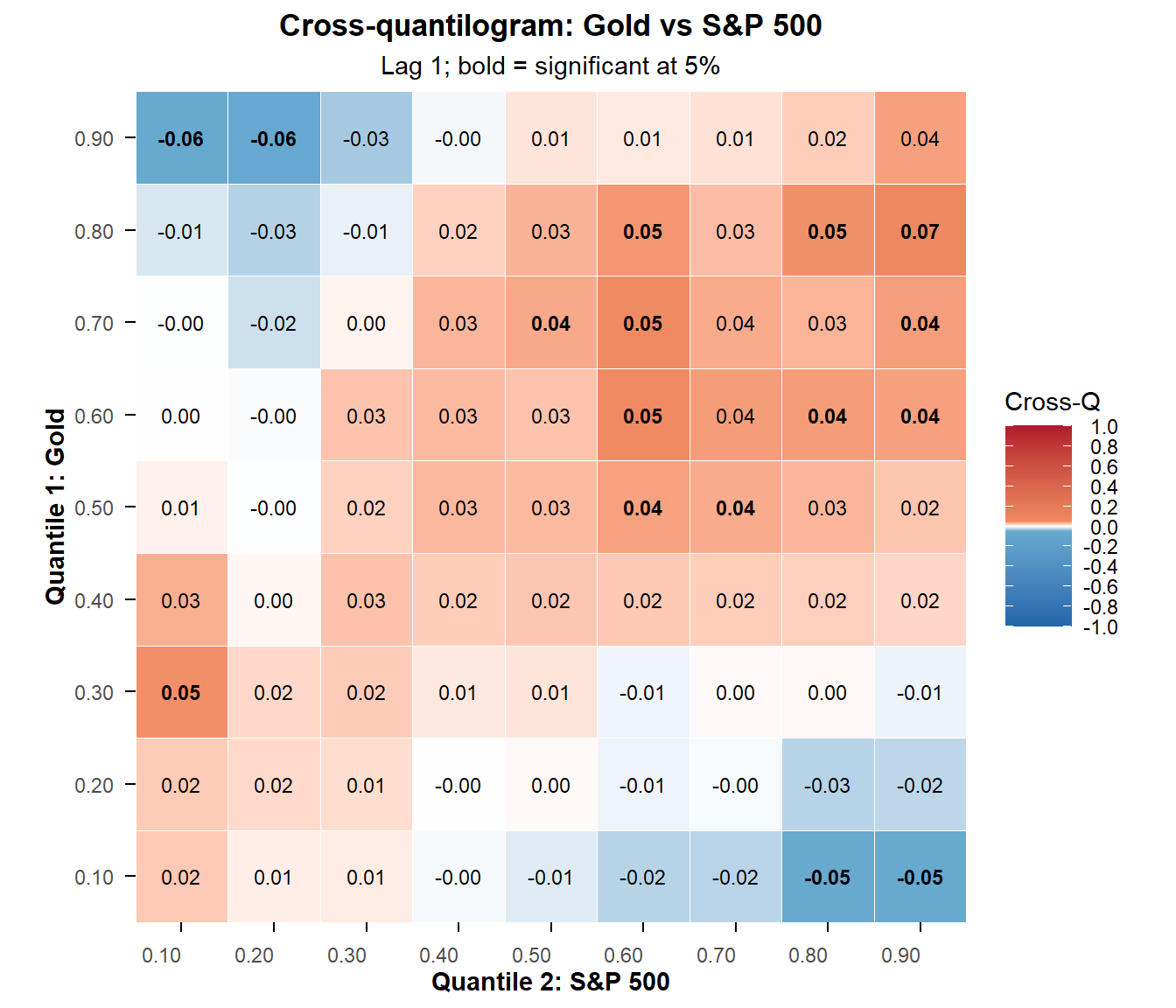
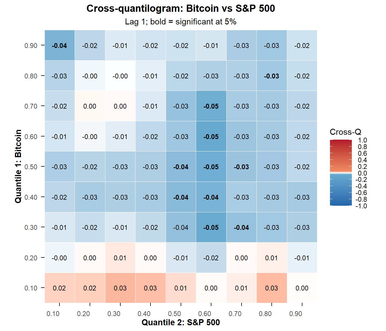
# Shared styling: the cross-quantilogram values are small, so the colour
# scale saturates at +/-0.05; bold values are significant at 5%.
heatmap <- function(df, var1, var2) {
  res <- crossq.heatmap(
    df, k, vec.q, B.size,
    var1_name = var1, var2_name = var2,
    title = paste("Cross-quantilogram:", var1, "vs", var2),
    subtitle = "Lag 1; bold = significant at 5%",
    colors = c("#2166AC", "#67A9CF", "white", "#EF8A62", "#B2182B"),
    color_values = c(-1, -0.05, 0, 0.05, 1),
    tile_border_color = "white", tile_border_width = 0.3, x_angle = 0
  )
  res$plot
}

# Gold (GLD) as predicted variable, S&P 500 (SP) as predicting variable
heatmap(hedgedata[, c("GLD", "SP")], "Gold", "S&P 500")

# Bitcoin (BTC) as predicted variable, S&P 500 (SP) as predicting variable
heatmap(hedgedata[, c("BTC", "SP")], "Bitcoin", "S&P 500")

The heatmaps show how dependence between the S&P 500 and gold or bitcoin varies across quantiles, indicating whether the hedging asset remains uncorrelated or negatively correlated during market stress.

4. Diversification benefit

# S&P 500 / gold portfolio, 90% in the S&P 500, 5% tail
diversification_benefit(hedgedata$SP, hedgedata$GLD, p = 0.05, w = 0.90)

[1] 0.3011936

# S&P 500 / bitcoin portfolio, 90% in the S&P 500, 5% tail
diversification_benefit(hedgedata$SP, hedgedata$BTC, p = 0.05, w = 0.90)

[1] 0.5089053

w is the weight on the first asset (here the S&P 500). The measure lies between 0 (no diversification benefit, as with perfectly correlated assets) and 1; higher values imply stronger diversification benefits.

References

Mujtaba, G., A. Siddique, N. Naifar, S. J. H. Shahzad. (2024). Hedge and safe haven role of commodities for the US and chinese equity markets. International Journal of Finance & Economics, 29, (2), 2381–2414.

Ali, S., E. Bouri, R. L. Czudaj, S. J. H. Shahzad. (2020). Revisiting the valuable roles of commodities for international stock markets. Resources Policy, 66, 101603.

Shahzad, S. J. H., E. Bouri, D. Roubaud, L. Kristoufek. (2020). Safe haven, hedge and diversification for G7 stock markets: Gold versus bitcoin. Economic Modelling, 87, 212–224.

Shahzad, S. J. H., E. Bouri, D. Roubaud, L. Kristoufek, B. Lucey. (2019). Is bitcoin a better safe-haven investment than gold and commodities? International Review of Financial Analysis, 63, 322–330.

Christoffersen, P., K. Jacobs, X. Jin, H. Langlois. (2018). Dynamic dependence and diversification in corporate credit. Review of Finance, 22, (2), 521–560.

Basher, S. A., P. Sadorsky. (2016). Hedging emerging market stock prices with oil, gold, VIX, and bonds: A comparison between DCC, ADCC and GO-GARCH. Energy Economics, 54, 235–247.

Han, H., O. Linton, T. Oka, Y.-J. Whang. (2016). The cross-quantilogram: Measuring quantile dependence and testing directional predictability between time series. Journal of Econometrics, 193, (1), 251–270.

Christoffersen, P., V. Errunza, K. Jacobs, H. Langlois. (2012). Is the potential for international diversification disappearing? A dynamic copula approach. Review of Financial Studies, 25, (12), 3711–3751.

Baur, D. G., T. K. McDermott. (2010). Is gold a safe haven? International evidence. Journal of Banking & Finance, 34, (8), 1886–1898.